Survey-Grade GNSS Corrections and Data Formats Explained
Your comprehensive guide to achieving centimeter-level accuracy with GNSS technology — RTK, NTRIP, RTCM MSM, PPP and CORS, demystified.
Introduction
High-precision GNSS positioning depends not only on the quality of the receiver but also on the correction data it applies. By default, a GNSS receiver operates in autonomous mode, using only raw signals from satellites. This provides accuracies of 1–5 m, sufficient for navigation but inadequate for surveying, agriculture, UAV mapping, or machine control.
To achieve centimeter-level accuracy, users rely on corrections transmitted from different sources. These corrections can be delivered via a local base station, a CORS network, or even from satellites. Depending on the method, corrections reach the rover over UHF/VHF radio, cellular (NTRIP), Wi-Fi, or L-band satellite links.
As an authorized CHCNAV dealer in Canada, Latnet Technologies Ltd. sees every day how the right correction service + data format selection impacts surveyors, farmers, machine control operators, and UAV teams. This article explores the main GNSS positioning modes, the factors influencing accuracy, and the data protocols (RTCM, MSM, CMR/CMRx, Leica, RINEX, BINEX, SSR) that power them.

Modern GNSS receivers enable centimeter-level accuracy for surveying and precision applications.
Positioning Modes and Correction Services
1) Autonomous GNSS
How it works: In autonomous (stand-alone) mode, the receiver calculates its position using only raw pseudorange measurements from GNSS satellites. No external corrections are applied to mitigate errors from the ionosphere, troposphere, satellite clocks, or orbital uncertainties.
Accuracy: Typically 1–5 m (95%), depending on receiver quality, atmospheric conditions, and satellite geometry.
Use cases: Car navigation, fleet tracking, recreational GPS, mobile devices.
Limitations: Not reliable for survey or machine control; errors worsen in urban canyons and under canopy; sensitive to ionospheric disturbances.
2) SBAS (Satellite-Based Augmentation Systems)
How it works: SBAS augments autonomous GNSS by broadcasting satellite clock, ephemeris, and ionospheric corrections from geostationary satellites. Corrections are generated by ground monitoring networks and uplinked to the SBAS satellite.
- WAAS — North America
- EGNOS — Europe
- MSAS — Japan
- GAGAN — India
Accuracy: 0.5–1 m horizontal, 1–3 m vertical.
Use cases: Aviation (ICAO), GIS mapping, mid-precision agriculture guidance.
Limitations: Regional coverage; not carrier-phase precise; not survey-grade.
3) Single-Base RTK (Real-Time Kinematic)
How it works:
- A GNSS base is installed over a known control point.
- The base streams raw carrier-phase + pseudorange observations to the rover, which computes differenced corrections.
Links: UHF/VHF radio, cellular modem, or Wi-Fi (UAVs).
Accuracy: 2–3 cm horizontal, 3–5 cm vertical within ~10–40 km, depending on atmosphere.
Use cases: High-precision surveying, construction staking, precision-ag machinery, UAV photogrammetry/LiDAR.
Limitations: Daily setup/maintenance; baseline-dependent (≈ 1 mm/km rule of thumb); radio line-of-sight constraints.
4) CORS / Network RTK
How it works:
- CORS are permanent, geodetic-grade receivers installed on stable monuments (buildings, pillars, towers).
- Observations stream to a central control server (NTRIP caster).
- The server computes corrections for the rover using one of:
- Nearest Base
- VRS (Virtual Reference Station)
- MAC (Master–Auxiliary Concept)
Accuracy: 2–3 cm horizontal, 3–5 cm vertical across the service area.
Use cases: National/provincial survey networks, agriculture, engineering projects needing long-term consistency.
Limitations: Requires cellular coverage; subscription-based; performance depends on station density and atmospheric modeling.
5) Satellite-Delivered Corrections (L-band PPP / PPP-RTK)
How it works: Global/regional services broadcast corrections over L-band via geostationary satellites. Rovers receive corrections directly — no local comms or cell coverage needed. Often PPP (Precise Point Positioning) or hybrid PPP-RTK / SSR approaches.
Examples: CHCNAV PointSky, Trimble RTX, NovAtel TerraStar, Leica SmartLink, Hemisphere Atlas.
Accuracy: Sub-meter quickly; 10–20 cm within minutes; 2–5 cm after 5–30 min of full convergence (tier-dependent).
Use cases: Offshore rigs, continental farming, remote resource exploration, UAVs beyond CORS coverage.
Strengths: Global/continental coverage; no cellular or radio infrastructure required.
Limitations: Unobstructed sky required; subscription-based; 5–30 min convergence; outputs typically in ITRF/global frame — requires Helmert transformation parameters and a velocity grid (e.g., NAD83(CSRS) in Canada) for local datum alignment.

RTK GNSS systems provide centimeter-level accuracy for surveying applications.
Ready to Upgrade from Autonomous or SBAS to Reliable cm-Level RTK?
Contact Latnet Technologies for a free consultation on integrating CHCNAV GNSS receivers into your workflow.
Get Professional ConsultationWhat Influences GNSS Accuracy? (Technical)
1) Satellite Constellations & Geometry
Geometry matters: wider, evenly distributed satellite coverage yields more robust solutions.
Dilution of Precision (DOP): a unitless factor describing how geometry amplifies position error.
- PDOP (Position DOP) — overall 3D quality
- HDOP (Horizontal) — X/Y
- VDOP (Vertical) — Z
- TDOP (Time) — clock bias
- GDOP (Geometric) — position + time
Typical thresholds:
- PDOP < 2 → Excellent (survey-grade)
- PDOP 2–4 → Acceptable for mapping/machine guidance
- PDOP > 6 → Poor, unreliable
Multi-constellation advantage: Using GPS, GLONASS, Galileo, and BeiDou together provides 30–40+ satellites in view, significantly lowering DOP, minimizing outages, and improving robustness under canopy or in urban canyons.
2) Multipath Effects
Definition: Multipath occurs when GNSS signals don't travel directly from the satellite to the antenna. Instead, they reflect off buildings, vehicles, water bodies, metallic surfaces, or even the ground before reaching the receiver. The delayed reflected signals combine with the direct path, creating biased pseudorange and carrier-phase measurements.
Error magnitude:
- Code pseudorange multipath: 0.5–5 m depending on environment and signal bandwidth
- Carrier-phase multipath: typically <5 cm, but still critical for RTK ambiguity resolution
- Frequency dependence: Narrowband signals (e.g., GPS L1 C/A) are more vulnerable than modern wideband signals (e.g., Galileo E5)
Environment impact:
- Urban canyons: severe, frequent reflections
- Forests: diffuse multipath from leaves and branches
- Open fields: minimal multipath, but vehicles and UAV frames can still reflect
Why it matters:
- Causes unstable positions in RTK
- Lengthens convergence in PPP/SSR
- Degrades vertical accuracy more than horizontal
- Can make real-time quality metrics (RMS, fixed/float ratio) misleading
Mitigation strategies:
- Hardware-based: choke-ring antennas; ground planes; geodetic-grade antennas with strong multipath suppression
- Signal processing: multipath-resistant correlators; modernized modulations (BOC/BPSK)
- Field practices: avoid reflectors; use elevation masks (e.g., 10° to exclude low, noisy signals); keep UAV antennas above props and reflective airframe parts
- Software/processing: SNR-based weighting; post-process with multipath detection filters
Bottom line: Multipath is often the largest error source in urban and construction environments. Good antenna + thoughtful placement + intelligent filtering can reduce it substantially — rarely entirely.

Multipath occurs when GNSS signals reflect off surfaces before reaching the receiver.
3) Atmospheric Delays
GNSS signals must pass through the ionosphere and the troposphere, both of which bend and slow the signal. These are among the most significant error sources.
Ionosphere (dispersive delay)
Cause: Free electrons interact with radio waves. The effect is frequency-dependent (dispersive): lower frequencies (e.g., GPS L1) are delayed more than higher ones.
Magnitude:
- On single-frequency receivers, errors can reach 10–50 m during strong solar activity
- Variability depends on time of day, season, latitude, and 11-year solar cycles
- Geomagnetic storms can cause sudden degradations
Mitigation:
- Dual-/triple-frequency receivers form ionosphere-free linear combinations, e.g.:
PIF = (f12·P1 − f22·P2) / (f12 − f22)
where P1 and P2 are pseudoranges measured on frequencies f1 and f2; the same combination form applies for carrier phase Φ.
- Network RTK interpolates ionospheric gradients from multiple bases
- PPP/SSR uses global iono models (IGS, Galileo HAS)
During geomagnetic storms, expect longer RTK initialization and slower PPP convergence; in severe cases, rescheduling critical work is safer.
Field note: Single-frequency (L1-only) receivers are hit hardest. For professional surveying, multi-frequency rovers like the CHCNAV i93 or i89 are essential.
Troposphere (non-dispersive delay)
Cause: Neutral atmosphere (temperature, pressure, humidity) slows signals equally across frequencies.
Magnitude:
- Zenith delay typically 2.3–2.5 m
- Mapping functions convert this to 10–20 m near the horizon
- Highly variable with local humidity and weather systems
Mitigation:
- Models: Saastamoinen, Hopfield, GPT2w
- Estimate ZTD (Zenith Tropospheric Delay) in PPP and advanced RTK filters
Field note: On long baselines, ionosphere dominates; for vertical accuracy, troposphere often rules. Network RTK / PPP with tropospheric estimation is key for engineering-grade heights.
4) Baseline Length (RTK)
Why distance hurts RTK: RTK cancels shared errors by differencing base/rover observations. As baseline increases, ionospheric, tropospheric, and orbit errors decorrelate, leaving larger residuals. Transport effects (radio latency/jitter) also scale with distance.
Rule of thumb: ~1 ppm baseline-dependent error → 1 mm/km after differencing.
- 10 km ≈ 1 cm
- 40 km ≈ 4 cm
- 60 km ≈ 6 cm (ambiguity fixing may become intermittent)
Baseline Length Impact on RTK Performance
| Baseline | Expected RTK Behavior | Recommended Strategy |
|---|---|---|
| 0–10 km | Rapid fixed; cm-level H/V | Single-base RTK; full multi-GNSS; MSM5/7; keep latency low |
| 10–20 km | Usually fixed; vertical more sensitive | Single-base OK; monitor iono/tropo; strong antenna and placement |
| 20–40 km | Slower fixes; occasional float; vertical noise | Prefer NRTK (VRS/MAC); ensure GLONASS 1230; consider higher elevation mask |
| 40–60 km | Intermittent fixing; frequent re-init | NRTK strongly recommended; otherwise SSR/PPP rather than forcing RTK |
| >60 km | Unreliable single-base RTK | SSR/PPP(-RTK) or relocate base / use a denser network |

RTK accuracy decreases with distance — fast and stable within 20 km, usable up to 40 km, and unreliable beyond 60 km.
Radio vs. cellular considerations:
- UHF/VHF radios: Both narrow (12.5 kHz) and wide (25 kHz) channels are common — narrow ones limit message sets/rates (e.g., 4800–9600 bps, fitting MSM4/5), while wider ones support higher baud rates like 19200 bps for richer MSM5/7 streams. Use efficient MSM subsets or proprietary formats if single-vendor. Line-of-sight is the real limiter; terrain kills range even if baseline is short.
- Cellular/NTRIP: Baseline isn't RF-limited — but latency/jitter directly affect ambiguity maintenance.
Field best practices (distance-sensitive):
- Pick the closest CORS or VRS mountpoint — don't just choose the "richest" stream
- Always include RTCM 1230 when using GLONASS in mixed-brand fleets
- For long baselines, avoid low elevation satellites; use SNR-based weighting if available
- On high-iono days, log RINEX for PPK validation even when running RTK
- For machine control, consider a temporary on-site base to guarantee short baselines and low latency
Bottom line: Long baselines fail because the shared errors stop being shared. Modern rovers like the CHCNAV i93 and i89 push the boundary with better tracking and continuity — but the real win at distance is Network RTK or SSR.
5) Receiver & Antenna Quality
Centimeter-level GNSS depends on both receiver electronics and antenna design.
Receivers (Processing & Tracking)
- Multi-frequency capability
-
All-constellation tracking
- GPS, GLONASS, Galileo, BeiDou, QZSS, NavIC → 30–40+ sats visible; lower PDOP; fewer dropouts; faster re-fix
-
Signal tracking under stress
- Advanced correlators handle weak signals, interference, and multipath better → fewer RTK dropouts on construction sites, farms, and forests
Antennas (Design & Impact)
-
Geodetic-grade integrated antennas
- Stable phase center; multipath suppression; factory PCO/PCV calibration
- Engineered to complement the GNSS front-end; consistent across constellations and corrections (MSM5/MSM7)
-
Survey-grade dome antennas (external)
- Rugged, portable, good multipath rejection; common in modular rover setups
-
Patch antennas (low-cost / UAV GNSS)
- Lightweight and cheap but unstable phase centers → cm-level biases
- More vulnerable to multipath and polarization mismatch
- OK for consumer navigation, GIS, and lightweight drones; not for survey-grade RTK unless paired with strong augmentation (e.g., PPK)
Field note: Cutting antenna corners is a top cause of bad heights. For professional work, integrated geodetic-grade receivers like CHCNAV deliver faster convergence, stable solutions, and resilience in tough environments. For UAVs, verify whether the GNSS antenna is survey-grade or a patch — this often explains large accuracy deltas.
6) Communication Link Stability
Even with great receivers and corrections, GNSS collapses if the correction stream doesn't arrive in time.
RTK Latency Budget
- Target <1 s average latency; absolute max <2 s
- Beyond that, the rover loses integer lock and drops to float or autonomous
- This is often the hidden culprit behind "random floats"
UHF/VHF Radio Links
Frequencies: Licensed 440–470 MHz; ISM 902–928 MHz (regional).
Channel spacing:
-
12.5 kHz (narrowband)
- Usable throughput: typically 4800–9600 bps
- Fits efficient formats (e.g., MSM4/5 for GPS+GLONASS)
- May struggle with full multi-constellation MSM7
-
25 kHz (wideband)
- Usable throughput: 9600–19200 bps
- Supports richer MSM5/7 multi-constellation streams
Line-of-sight: Terrain, vegetation, and buildings attenuate quickly.
Range: 3–10 km typical with short antennas; 20–30 km with tall masts or repeaters.
Practical tip: On 12.5 kHz, trim unnecessary constellations or signals to reduce stream size.
Cellular (NTRIP over 3G/4G/5G)
- Standard for CORS/Network RTK delivery
- Protocols: NTRIP v1 (HTTP), NTRIP v2 (HTTPS/TLS)
- Latency depends on mobile network quality; spikes >2 s cause rovers to drop fix
Best practices:
- Use multi-network SIMs for rural coverage
- Enable auto-reconnect in field apps (e.g., CHCNAV LandStar)
- Monitor correction age and latency indicators in real time
Wi-Fi (2.4 / 5 GHz)
- Short-range, high-speed, low-latency
- Common in UAV workflows (ground → drone)
- Range: <500 m unless extended with directional antennas
- Vulnerable to interference in crowded environments
L-band Satellite (PPP / PPP-RTK)
- Wide-area corrections via geostationary satellites
- Bandwidth: ~600–1200 bps, optimized for SSR/PPP
Strengths: Global/continental coverage; no cellular or radio infrastructure needed.
Limitations: Unobstructed sky required; subscription; 5–30 min convergence.
Use cases: Offshore rigs, continental farming, UAVs beyond cell range.
Communication Link Comparison
| Link Type | Channel Spacing / Baud | Usable Payload | Fits Best |
|---|---|---|---|
| UHF 12.5 kHz | 4800–9600 bps | ~600–1200 bps | RTCM MSM4/5 |
| UHF 25 kHz | 9600–19200 bps | ~1800–2400 bps | RTCM MSM5/7 (multi-constellation) |
| Cellular (NTRIP) | >10 kbps | Practically unlimited | RTCM MSM7, SSR |
| Wi-Fi | Mbps | Any | UAV corrections |
| L-band Satellite | ~600–1200 bps | SSR/PPP streams | PPP-RTK services (PointSky, RTX, TerraStar, SmartLink) |
Bottom line: The receiver is only as good as its comms link. With CHCNAV receivers you can confidently run UHF, cellular, Wi-Fi, and L-band — but plan channel width and baud to avoid overload, especially on narrowband UHF.
Struggling with multipath or atmospheric delays in your projects?
Unlock next-level GNSS performance with CHCNAV — reach out to Latnet to get started.
Contact UsInteroperability Gotchas (Save a Ton of Pain)
- Base–Rover message bundles: In single-vendor base/rover setups (e.g., CHCNAV iBase → i93), you don't pick individual RTCM messages — the base outputs a fixed bundle. Same brand? It just works. Mixing brands? If the rover can't decode that bundle (e.g., ignores MSM7), you may never get a fix. Use proper settings to mix brands.
- Network RTK mountpoints: Unlike base–rover, CORS/NTRIP services publish multiple mountpoints (legacy 1004/1012, MSM5, MSM7). You must choose one your rover supports. Older gear may only handle legacy messages; modern receivers like CHCNAV take full MSM7. Pick wrong → wasted time.
- GLONASS inter-frequency biases: Mixed-brand RTK needs RTCM 1230. Without it, GLONASS observations probably won't align and ambiguities won't resolve.
- Antenna descriptors: Always broadcast 1007/1008 or 1033 (antenna type + serial) so the rover applies the correct APC/PCV corrections. Wrong antenna models = wrong heights.
- Latency budget: Keep <2 s end-to-end. Higher latency = float or no fix. Design redundancy (dual-SIM, buffered NTRIP) if coverage is shaky.
- Datum/epoch mismatch: Mixing frames (e.g., ITRF2014 vs NAD83(CSRS)) without transformation → meter-level offsets. Always confirm datum and epoch with your network provider.
Data Stream Comparison
| Stream Type | What's Inside | Approx. Data Rate (1 Hz, per constellation) | Notes |
|---|---|---|---|
| Legacy 1004/1012 | GPS + GLONASS dual-freq full obs | 250–400 bps | Common on older radios; less efficient |
| MSM4 | Code + Carrier + CNR (no Doppler) | 350–700 bps | Good detail vs size; robust RTK at lower bandwidth |
| MSM5 | Code + Carrier + CNR + Doppler | 400–800 bps | Widely used in CORS; CNR aids QC and multipath detection |
| MSM7 | Code + Carrier + CNR + Doppler (high-resolution) | 500–1000 bps | Richest dataset; heavier load |
| CMRx (Trimble) | Proprietary compressed multi-GNSS | ~200–400 bps | Highly efficient; brand-locked |
| Leica proprietary | Compressed stream | ~200–400 bps | Efficient within SmartNet; no cross-brand use |
Practical Selection Guide (Actionable)
| Scenario | Recommended Path | Why It Works |
|---|---|---|
| Mixed-brand survey fleet (Canada) | RTCM 3.x MSM5 via CORS (NTRIP) | MSM5 is the safest universal choice — all major brands decode it. CHCNAV GNSS receivers handle MSM5 seamlessly. |
| High-end survey (where MSM7 is offered) | MSM7 mountpoint | Full high-resolution observables (code, carrier, Doppler, CNR). Modern receivers like CHCNAV fix faster and deliver stronger QC. |
| Trimble-only workflows | CMRx | Extremely bandwidth-efficient in Trimble stacks; proprietary. |
| Leica-only workflows | Leica compressed or RTCM MSM | Leica formats save bandwidth; for mixed fleets, fall back to RTCM for interoperability. |
| Remote/offshore / no cellular | L-band PPP / PPP-RTK (SSR) | PointSky/RTX/TerraStar/Atlas/SmartLink converge to 2–5 cm without ground infrastructure. |
| UAV mapping near site | Single-base RTK (RTCM over UHF/Wi-Fi) + RINEX PPK backup | Real-time efficiency + post-processed redundancy for deliverables. |
| Large-scale agriculture & machine control | Network RTK MSM5 | Region-wide coverage; stable 1–2 cm pass-to-pass. |
Latnet Pro Tip: At Latnet Technologies Ltd., we routinely deploy CHCNAV GNSS receivers on MSM5 streams for maximum interoperability across Canadian CORS. Where MSM7 is available, we switch to it to unlock faster ambiguity resolution and richer signal-quality indicators.
Base Setup Best Practices (That Actually Matter)
-
Monument & Sky View
- Install the base on a stable monument (survey control point, concrete pillar, reinforced building mount) or at least a rigid tripod/tribrach.
- Maximize sky view with a clear horizon.
- Elevation mask: 10–15° typical in open sky; 20–30° in multipath-heavy sites (urban canyons, reflective surfaces, dense vegetation).
- Avoid nearby reflectors (metal roofs, water, vehicles).
-
Reference Coordinates (Datum + Epoch)
- Always tie your base to a known reference: a published survey monument (correct datum/epoch) or static PPP (e.g., NRCan CSRS-PPP in Canada).
- Document datum and epoch (e.g., NAD83(CSRS) epoch 2010.0).
-
Antenna Height Measurement
- Define the reference clearly: bottom of antenna mount, lever point, or slant height to marker.
- Avoid generic "ARP" unless your calibration file references it.
- Record the method in the field log — 5 mm mistakes propagate everywhere.
-
Antenna Models & Correction Formats
- Ensure the base broadcasts antenna metadata (RTCM 1007/1008 or 1033) so the rover applies the correct PCV.
- Same-brand workflows (e.g., CHCNAV iBase + i93): you don't choose individual messages — the devices exchange a compatible bundle automatically; just match the format family (RTCM/CMRx/Leica).
- Mixed-brand fleets: stick to RTCM for maximum interoperability.
-
RINEX Logging (Always On)
- Always record base data in RINEX for PPK, QA/QC, and forensics.
- Archive systematically (station/year/month hierarchy).
-
Health Monitoring & Diagnostics
- Continuously track: latency (<2 s), # of satellites used, PDOP/HDOP/VDOP, residuals/fix ratio, radio RSSI or cellular stability.
- High-end receivers like CHCNAV include monitoring for QC.
-
Check-ins with the Rover
- After base setup, occupy the base point with the rover (especially if the rover is IMU-equipped) to validate antenna height and coordinates.
- Check in on another known point to confirm the entire chain (datum/epoch, geoid model, antenna model, height entry) is correct.

A proper GNSS base setup ensures stable positioning — maximize sky view, apply a 10–15° elevation mask, avoid reflectors, and record precise antenna height and RINEX data.
Troubleshooting Quick Wins (Field-Proven)
No Fix / Stuck in Float
- Confirm rover supports the MSM level (fall back to MSM5 if MSM7 isn't decoded)
- Verify correction data format (e.g., RTCM, CMRx)
- Check if corrections are being received (monitor correction age in software)
- Verify radio frequency, protocol (e.g., TRIMTALK 450S, SATEL, CHC), and settings for UHF/VHF
- Ensure latency < 2 s
- Include GLONASS RTCM 1230 in mixed-brand workflows
- Inspect sky view — obstructions or multipath can mimic "bad corrections"
Meter-Level Offset
- Datum/epoch mismatch (e.g., ITRF vs NAD83(CSRS)) or wrong geoid
- Check project CRS and geoid on the rover/controller
- Reconfirm base coordinates and epoch with the provider
Bad Heights
- Wrong antenna height entry (slant vs vertical) or wrong reference
- Antenna model/PCV doesn't match what the base broadcasts
- Re-occupy a known point to validate verticals
Radio Dropouts / Unstable Link
- 12.5 kHz narrowband overruns → reduce message set (drop extra constellations or signals) or lower update rate
- Scan 400–470 MHz for interference (telemetry, repeaters)
- Move to 25 kHz wideband or cellular NTRIP if persistent
UAV Timing "Chatter"
- Some UAV controllers expect 5–10 Hz correction updates for smooth kinematics
- Increase update rate if supported
Data Formats and Protocols for GNSS Corrections
1) RTCM (Radio Technical Commission for Maritime Services)
Overview: Open, international standard for real-time GNSS corrections; maintained by RTCM SC-104.
Evolution:
- RTCM 2.x (1990s): GPS → GLONASS; large messages; legacy radios
- RTCM 3.x (2004–present): Compact, modular; supports GPS/GLONASS/Galileo/BeiDou/QZSS/NavIC and multi-frequency (L1/L2/L5/E5/B1/B2…); standard for CORS/NTRIP and even SSR delivery
Representative message types (RTCM 3.x):
- 1004 / 1012: Legacy full obs (GPS / GLONASS)
-
MSM observation families (1071–1137):
- 1071–1077 — GPS
- 1081–1087 — GLONASS
- 1091–1097 — Galileo
- 1101–1107 — SBAS
- 1111–1117 — QZSS
- 1121–1127 — BeiDou
- 1131–1137 — NavIC/IRNSS (added in newer revisions)
- 1005 / 1006: Reference station coordinates (ECEF)
- 1007 / 1008 / 1033: Antenna/receiver descriptors + serials (phase center)
- 1019 / 1020 / 1045 / 1046: Broadcast ephemerides (GPS / GLO / GAL / BDS)
- 1230: GLONASS code-phase bias (critical for interoperability)
- 1057–1068: SSR orbit / clock / bias / atmosphere
Strengths: Open, extensible, widely adopted across CHCNAV, Trimble, Leica, Topcon, Septentrio.
Efficiency vs proprietary: Much smaller than 2.x but heavier than CMRx or Leica streams. Typical 250–600 bps per constellation (varies with sats / signals / rate).
Use cases: CORS/NTRIP, survey rovers, ag guidance, machine control, UAV mapping.
Limits: Bandwidth on older radios; configuration complexity (message mismatch issues).
RTCM MSM (Multiple Signal Messages)
Why MSM: Older RTCM 3.x messages were constellation/signal-specific; MSM unifies representation across constellations and signals. Per the official RTCM 10403.x standard, MSM types are defined as follows (note: MSM4 and MSM6 do not contain Doppler — only the odd-numbered MSM5 and MSM7 do):
| MSM Level | Observables Included | Benefits / Use Cases |
|---|---|---|
| MSM1 | Pseudorange (code) only | DGNSS uses; ultra-light; legacy and integrity checks |
| MSM2 | PhaseRange (carrier-phase) only | Niche; rarely deployed in practice; very light bandwidth use |
| MSM3 | Pseudorange + PhaseRange | Minimum recommended for relative positioning / RTK with reduced data |
| MSM4 | Pseudorange + PhaseRange + CNR (no Doppler) | Strong RTK with good efficiency; ideal for bandwidth-constrained UHF links |
| MSM5 | Pseudorange + PhaseRange + CNR + Doppler | Widely used in CORS networks; SNR aids QC and multipath detection |
| MSM6 | Pseudorange + PhaseRange + CNR (high-resolution, no Doppler) | Extended-precision variant of MSM4; less common in practice |
| MSM7 | Pseudorange + PhaseRange + CNR + Doppler (high-resolution) | Premium full observables; best for multi-GNSS RTK / PPP-RTK and UAV mapping |
2) CMR, CMR+, and CMRx (Trimble)
- CMR (original): 1990s; compact GPS L1/L2 only; radio-friendly
- CMR+: Adds GLONASS; legacy networks still use it
- CMRx: Modern multi-GNSS / multi-frequency; often ~50% less bandwidth than comparable RTCM MSM; Trimble-only
Strengths: Excellent efficiency over narrowband radios; fast init in Trimble stacks.
Limits: Proprietary; limited cross-brand support (CMRx essentially Trimble-only).
Use cases: Trimble base–rover ecosystems; private networks.
3) Leica Proprietary Formats
Overview: Leica compressed streams (often referred to as 4G/5G generations) optimized for SmartNet and Leica rovers.
Strengths: Very compact; robust within Leica ecosystem.
Limits: Vendor lock-in; closed format.
Use cases: Leica SmartNet; single-vendor firms.
4) RINEX (Receiver Independent Exchange Format)
Overview: Open ASCII standard for vendor-neutral sharing and processing of raw observations; maintained by IGS.
Versions:
- RINEX 2.x: GPS / GLONASS; legacy
- RINEX 3.x: All constellations + modern signals; richer metadata (current 3.05, 2020)
- RINEX 4.x: Released by IGS in December 2021; current version is RINEX 4.02 (2024). Modernizes navigation messages to support multi-GNSS, system data messages (ionospheric corrections, Earth orientation parameters, system time offsets), and pico-second-resolution epoch tagging
Structure:
- .O — observations (code, carrier, Doppler, SNR) per epoch/satellite
- .N, .G, .L, .C, … — broadcast ephemerides
- .M — meteorological (P/T/RH)
- SP3 — precise orbits/clocks (paired for PPP)
Applications: PPK, PPP (NRCan CSRS-PPP), archiving (NRCan / NOAA), geophysics / tectonics / atmosphere.
Pros: Vendor-neutral; human-readable; universal in research and government.
Cons: Large files; not for real-time; conversion from proprietary raw formats (.dat / .t02 / .m00 / .raw) often required.
5) BINEX (Binary Exchange Format)
Overview: Open binary format by UNAVCO; designed for both streaming and archiving.
Pros: Flexible; efficient vs ASCII.
Cons: Niche outside academia; limited native support in commercial hardware.
Use cases: Scientific networks; advanced research.
6) SSR (State Space Representation)
Overview: Instead of observation-differencing, SSR transmits error states: orbit, clock, code/phase biases, atmosphere.
Advantages: Scales to continental and global coverage; efficient for PPP-RTK; reduces convergence vs classic PPP.
Standards & adoption: Defined in RTCM (messages 1057–1068); used by Galileo HAS, CHCNAV PointSky, Trimble RTX, Leica SmartLink, and others.
Use cases: L-band and IP-delivered PPP-RTK services.
Frequently Asked Questions
What is the difference between RTK and PPP GNSS corrections?
RTK (Real-Time Kinematic) uses observation-space corrections from a nearby base or CORS network and delivers 1–3 cm accuracy almost instantly, but requires a local reference within roughly 40 km. PPP (Precise Point Positioning) uses state-space corrections — orbit, clock, atmosphere — broadcast globally over L-band or IP, works anywhere with sky view, but typically needs 5–30 minutes to converge to 2–5 cm accuracy.
How accurate is RTK GPS surveying?
Survey-grade RTK GNSS achieves 2–3 cm horizontal and 3–5 cm vertical accuracy within roughly 10–40 km of the base station, assuming a multi-frequency, multi-constellation receiver, a stable correction link with under 2 seconds of latency, and a clear sky view.
What is the difference between RTCM MSM5 and MSM7?
Both MSM5 and MSM7 carry pseudorange, carrier-phase, Doppler, and CNR observations. MSM7 is the high-resolution version, providing extended-precision values used for premium multi-GNSS RTK and PPP-RTK. MSM5 uses standard precision and is widely deployed in CORS networks because it delivers excellent RTK quality at lower bandwidth than MSM7. Note that MSM4 and MSM6 do not contain Doppler.
What is NTRIP and how does it deliver GNSS corrections?
NTRIP (Networked Transport of RTCM via Internet Protocol) is the standard for streaming GNSS corrections over the internet. A CORS network publishes correction streams (mountpoints) on an NTRIP caster, and rovers connect over cellular data using NTRIP v1 (HTTP) or v2 (HTTPS/TLS). Latency under 2 seconds is critical for stable RTK fixes.
How far can an RTK base station broadcast corrections reliably?
Single-base RTK delivers reliable centimeter-level fixes up to about 20 km, remains usable up to 40 km with some vertical degradation, and becomes intermittent beyond 60 km as ionospheric and tropospheric errors stop being shared between base and rover. For longer baselines, switch to Network RTK (VRS/MAC) or PPP-RTK.
Why do I need RTCM message 1230 when using GLONASS?
GLONASS uses FDMA, where each satellite transmits on a slightly different frequency. Different receiver brands have different inter-frequency code biases. RTCM message 1230 broadcasts the base receiver's GLONASS code-phase biases so a mixed-brand rover can align observations and resolve ambiguities. Without 1230, GLONASS ambiguities often will not fix in mixed-brand setups.
Which GNSS correction service is best for remote work without cellular coverage?
L-band PPP and PPP-RTK services such as CHCNAV PointSky, Trimble RTX, NovAtel TerraStar, Leica SmartLink, and Hemisphere Atlas broadcast corrections from geostationary satellites. They work continent-wide without cellular or radio infrastructure, converging to 2–5 cm in 5–30 minutes — ideal for offshore, remote agriculture, and exploration work beyond CORS coverage.
Closing Thoughts
GNSS corrections aren't one-size-fits-all. Accuracy depends on satellite geometry, atmosphere, baseline length, receiver and antenna quality, and communication stability — and every link must be tuned correctly. At Latnet Technologies Ltd., we deploy CHCNAV GNSS solutions to simplify interoperability, maximise efficiency across UHF, cellular, and L-band links, and help Canadian surveyors, precision-ag operations, and machine-control teams achieve dependable centimetre-level results. Whether you're setting up a private base, connecting to a provincial CORS network, flying UAV LiDAR missions, or operating in obstructed environments — choosing the right correction service and data format is the difference between frustration and flawless outcomes.
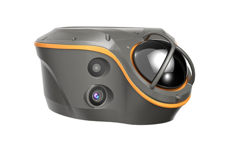
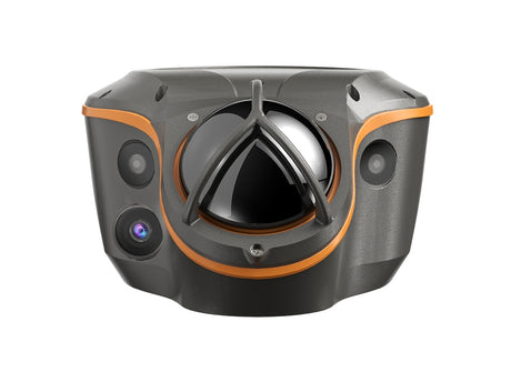
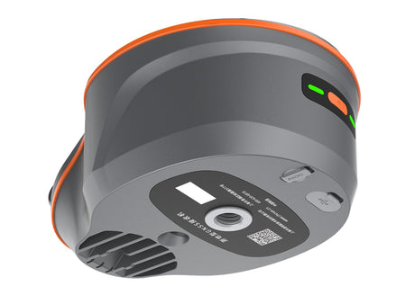
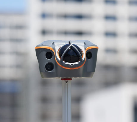
What's more, manufacturers like CHCNAV are now integrating high-precision GNSS receivers with LiDAR and visual-sensor technology in a single instrument. Take the CHCNAV ViLi i100 for example — a Visual-LiDAR GNSS-RTK receiver that combines advanced satellite filtering, LiDAR point-cloud scanning, and SLAM-based positioning to deliver consistent centimetre-level accuracy even in challenging GNSS-denied or obstructed environments.
At the end of the day, precision is not just about satellites — it's about the entire ecosystem working in harmony. From the CHCNAV i93 and i89 rovers to the new ViLi i100 GNSS + LiDAR integration, Latnet Technologies Ltd. continues to help professionals across Canada build smarter, more reliable, and future-ready positioning workflows.
Let's Make Your Next Project Seamless
Schedule a free CHCNAV GNSS demo with Latnet today and see cm-level precision in action.
Schedule a Free Demo
A surveyor, UAV, and tractor all rely on GNSS satellites to achieve precise positioning — illustrating the versatility of modern CHCNAV solutions across surveying, mapping, and precision agriculture.